Here you will find out latest app notes.
This application note discusses the Importance of Ferrite Beads for in Electromagnetic Interference (EMI) and using these Models in High Speed designs. This document also gives guidelines on the selection of a Bead model.
Ferrite Beads are passive electric components that suppresses high frequency noise in electronic circuits.
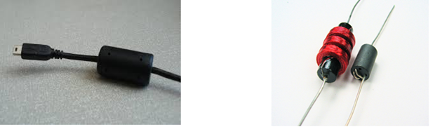
Figure 1: Images of EMI Filters
Ferrite Beads were traditionally used to make high frequency low pass filters and to keep transistors from oscillating. With today’s high performance systems, it is important to consider the bead’s real properties and to analyze the resulting bead circuit.
Popular Ferrite Bead Models of Fair-Rite #43 and #73 are discussed in this document.
#43 is a Nickel-Zinc Ferrite Bead used for suppression of conducted EMI from 20 MHz to 250 MHz and #73 is a Manganese-Zinc Ferrite Bead to suppress conducted EMI frequencies below 50 MHz.
The most important factors in ferrite bead-based design are:
• Impedance vs. bead size
• Impedance vs. frequency
• Impedance vs. DC current bias
• Impedance vs. number of turns on the bead
Ferrite Beads have the following advantages:
1. EMI Suppression
2. Improving Supply decoupling
3. Controlling parasitic Oscillations
4. Reducing RF Coupling
Impedance of a bead depends on the material and dimensions of the bead.
In the following Fig.2, Bead #2 has more inductance than Bead #1.
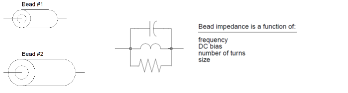
Figure 2: Impedance of Bead
Two different approaches to model Ferrite Beads in PSpice has been described below.
Ferrite beads used for power supply decoupling represent a difficult modeling problem for those involved in SPICE circuit simulations. The bead’s frequency-dependent nonlinear and non-monotonic behavior are particularly difficult to model.Eventually, the best recourse is to use simple L-R type equivalent circuit models. Accurate modeling and simulation of ferrite beads over a wide range is possible. To model the bead, a voltage-controlled current source (VCCS) behavioral model is used in such a way that the source’s terminals appear as an impedance. The source’s current is controlled by its terminal voltage as follows:
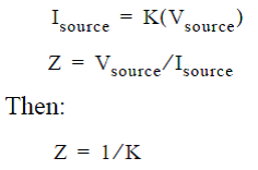
Thus, the terminal impedance (Z) is the reciprocal of the source’s scale factor (K). The listing illustrates this concept for a sub circuit model of the Fair-Rite 2673000101 ferrite bead.Data is entered into the table as frequency, magnitude of 1/Z in decibels, and the angle of 1/Z in degrees.
.SUBCKT BEAD73 1 2
GBEAD 1 2 FREQ { V(1, 2) }= ((1K,40.5,-89.9)
+ (10k, 20.6, -89.5)
+ (100k, 0.9, -80.5)
+ (1meg, -20.4, -59.5)
+ (2meg, -23.4, -46.0)
+ (3meg, -24.7, -39.1)
+ (5meg, -25.4, -36.9)
+ (7meg, -26.2, -35.9)
+ (10meg, -27.7, -34.6)
+ (20meg, -30.0, -23.0)
+ (30meg, -30.3, -16.5)
+ (40meg, -30.0, -12.0)
+ (50meg, -29.7, -08.0)
+ (60meg, -29.6, -06.5)
+ (70meg, -29.6, -06.3)
+ (80meg, -29.6, -06.2)
+ (100meg, -29.6, -06.6)
+ (200meg, -29.7, -09.5)
+ (1000meg, -32.0, -26.0))
RBEAD 1 2 200
.ENDS BEAD73
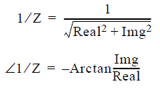
If ferrite bead data is unavailable in an impedance magnitude and angle format, then the impedance magnitude and angle should be computed as:
Resistor RBEAD in the listing was included to reduce the Q of the bead and supply a real shunt impedance around the VCCS. RBEAD is determined empirically with the VCCS frequency table coefficients to provide a good representation of the bead’s frequency dependent behavior.
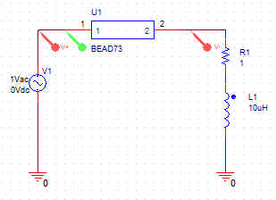
Figure 3: Circuit Design for BEAD73_1
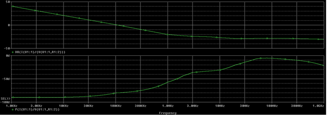
Figure 4: Simulation results for BEAD73_1
The second method of modelling a Ferrite Bead depends on its Physical core properties contribute to the inductance/impedance:
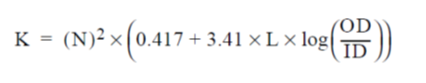
K is the impedance scaling factor,
L is the bead length,
OD is the outside diameter of the bead in inches,
ID is the inside diameter of the bead in inches.
N is the number of wire turns on the bead.
Note: A bead measuring 0.43” x 0.2” x 0.08” (Len, OD, ID) was used as the standard bead to which all others were scaled.
Ferrite bead’s electrical properties can be modeled by a simple parallel L-R-C circuit. By properly picking the L, R, and C components, a good fit can be made to the actual bead’s performance. These are generally the only components that need to be changed in the model to simulate different bead materials.
Here is an example ferrite bead model.
.SUBCKT BEAD_73 Z1 Z2
+ PARAMS:
+ ID_Bead=0.08
+ OD=0.2
+ L=0.43
+ N=1
* * Impedance multiplier * *
EOUT Z1 10 VALUE={V(GEOM)*V(BIAS)*V(ZREF)}
VSENSE 10 Z2 DC 0
GCOPY 0 ZREF VALUE={I(VSENSE)}
* * Impedance correction for bead size and number of turns * *
EGEOM GEOM 0
+ VALUE={N*N*(0.417+3.41*L*LOG10(OD/ID_Bead)) }
RGEOM GEOM 0 1MEG
* * Impedance correction for DC current bias, turns and diameter * *
EBIAS BIAS 0 TABLE {I(VSENSE) * N / (OD/0.2)} =
+ (-14,0.09)(-10.0,0.14)(-8.0,0.17)(-6.0,0.23)(-4.0,0.37)
+ (-2.0,0.77) (-1.0, 0.9) (0.0,1.0) (1.0,0.9) (2.0,0.77)
+ (4.0,0.37) (6.0,0.23) (8.0,0.17) (10.0,0.14) (14,0.09)
LBEAD ZREF 0 3U
RBEAD ZREF 0 111
CBEAD ZREF 0 {1.4P*N}
.ENDS
The bead is modeled in PSpice by using a basic impedance multiplier. The Circuit Design is shown in the Figure below. The circuit operates by sensing the AC current flowing through the bead and producing the voltage that relates to the correct impedance for that AC current and frequency.
The equation for this is Vout = Z x Iin
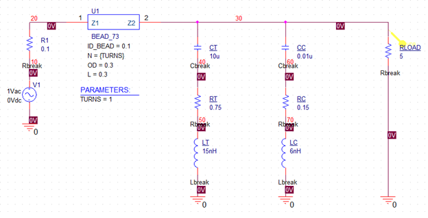
Figure 5: Circuit Design for bead73_1
To make this equation applicable to all circuit configurations of a bead, EOUT takes inputs from the geometry of the bead, DC bias level, number of turns, and the reference bead impedance to produce the correct equivalent impedance.
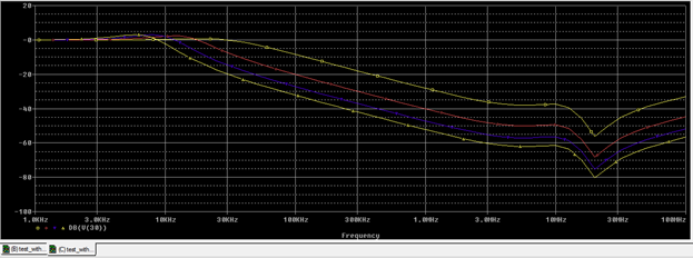
Figure 6: Simulation results for bead73_1
Inferences
The impedance correction for bead size is exactly like equation (1). The correction for DC bias does not fit well to a reasonable polynomial curve, so a lookup table is used to reduce the effective bead impedance with DC bias current. This method is usually preferable anyway. A lookup table has very well-defined values for points outside the bounds of the table, whereas a high-order polynomial may yield surprising outputs when inputs are well beyond the data used to fit the polynomial.
The lookup table for DC bias correction is further scaled by a factor that relates to the outside diameter of the bead. The larger the bead diameter, the more DC bias current it can accept before saturation. Conversely, if the number of turns is increased on the bead, the current it can support before saturation is reduced proportionally to N.
The last non-ideal correction for the bead is the CBEAD factor that relates to the turns on the bead. The inductance of the bead increases by N2, but the effect of the extra windings on the core increases the high frequency capacitance proportionally to N. The bead capacitance is first order corrected by multiplying by the number of turns, N.
All of these inputs are multiplied together at EOUT to produce the proper impedance for the bead. The model is valid for any analysis type and has exhibited no numerical instability in any of the dozen or so test circuits tried.
The subcircuit listing for the Fair-Rite #43 bead model. The subcircuit listing for the #73 bead model is similar; however, the following statements must be substituted for EBIAS, LBEAD, RBEAD, and CBEAD:
EBIAS BIAS 0 TABLE {I(VSENSE) * N / (OD/0.2)} =
+ (-14,0.09)(-10.0,0.14)(-8.0,0.17)(-6.0,0.23)(-4.0,0.37)
+ (-2.0,0.77) (-1.0, 0.9) (0.0,1.0) (1.0,0.9) (2.0,0.77)
+ (4.0,0.37) (6.0,0.23) (8.0,0.17) (10.0,0.14) (14,0.09)
LBEADZREF 0 3U
RBEADZREF 0 111
CBEADZREF 0 {1.4P * N}
Beads are used in many situations today to control EMI. One of the more useful configurations is to provide power supply decoupling on a per board basis. A typical expression is shown above. This is a standard circuit that may be used on a digital or analog PCB power entry. The bead used is a 0.3 OD x 0.1 ID x 0.3 L #73 core; the capacitors are modeled for series resistance and inductance as described in reference [2].
The resulting filter response is plotted versus the number of turns on the bead. An interesting thing happens with this circuit. As the number of turns is increased, the filter attenuation increases at high frequencies as expected; but at 10 kHz, the Q of the first pole also increases. This results in more peaking in the filter response which may or may not cause a problem for the circuit. It is, however, nice to know the full ramifications of increasing turns on the bead.
It can also be seen that increasing the turns on the bead above two does not significantly increase the filter rejection. This is due to the effects of the DC bias increasing proportionally to N.
The core can only support so many amp-turns before saturation—hence, the diminishing returns of attenuation as the turns are increased above a certain point.
The Fair-Rite #43 and #73 bead models presented in this article contains the equivalent schematics and symbol files for use in Schematics-based Design.
[1] Fair-Rite Soft Ferrites, 11th edition catalog, POB J, One Commercial Row, Wallkill, NY 12589
[2] Hageman, S. “Improve Simulation Accuracy When Using Passive Components,” The Design Center Source, April 1994, MicroSim Corporation, Irvine, CA.
[3] Acknowledgments: Special thanks go to William Kimmel of Kimmel Gerke Associates for laying the groundwork for modeling EMI ferrites in his article, “Wide Frequency Impedance Modeling of EMI Ferrites,” published in the IEEE 1994 Symposium on EMC. Mr. Kimmel is a well known EMI/EMC consultant and lecturer.
© Copyright 2015 Cadence Design Systems, Inc. All rights reserved. Cadence, the Cadence logo, and Spectre are registered trademarks of Cadence Design Systems, Inc. All others are properties of their respective holders.
1766 12/13 CY/DM/PDF
Copyright © 2020 Cadence Design Systems, Inc. All rights reserved.