Here you will find out latest app notes.
This application note will illustrate the method of creating nonlinear resistors using Analog Behavioral Modeling by creating the transfer function for a linear conductance. A conductance can be thought of as a voltage-controlled current source: the current between its nodes is a constant, times the voltage across those same nodes. For example:
GCOND A B VALUE = {V(A,B)*0.1}
Where A and B represent the positive and negative terminal nodes of the voltage source V2.
This represents a linear conductance with a value of 1 milli-ohm (that is, a 1m ohm resistor). The controlling nodes are the same as the output nodes.
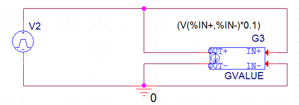
Figure 1: linear Conductance
For a nonlinear conductance the appropriate nonlinear function is used, but the device still has the same controlling and output nodes:
GSQ A B VALUE = {V(A,B)*V(A,B)*V(A,B)*1}
Where A and B represent the positive and negative terminal nodes of the voltage source V13.
GSQ has a small-signal conductance of 3×1×V(A,B)2. (The small-signal conductance is the derivative of the transfer function.)
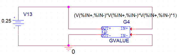
Figure 2: Quadratic Conductance
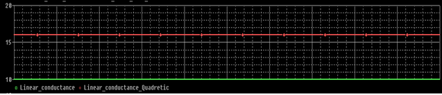
Figure 3: Simulation Results
Any nonlinear resistance can be expressed as a nonlinear conductance by inverting the transfer function. Sometimes, however, it is convenient to implement it directly. This can be done by noting that a resistor is a current-controlled voltage source. For example,
ERES A 4a VALUE = {I(VSENSE)*{10-1}}
VSENSE 4a B
Where A and B represents the positive and negative terminal nodes of V8.
This represents a linear resistor with a value of 1 kilo-ohm. VSENSE is needed to measure the current through ERES.
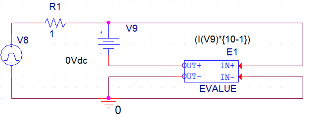
Figure 4: Linear Resistor
A quadratic resistor is then:
ERES A 4a VALUE = {PWRS(I(VSENSE),2)*{10-1}}
VSENSE 4a B
Where A and B represents the positive and negative terminal nodes of V12.
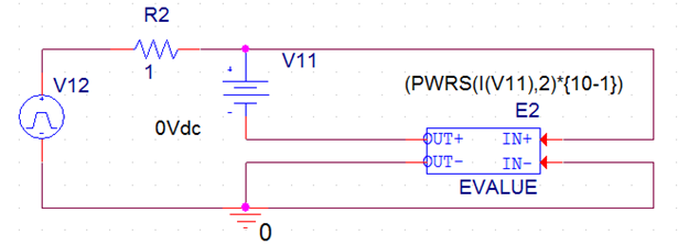
Figure 5: Quadratic Resistor
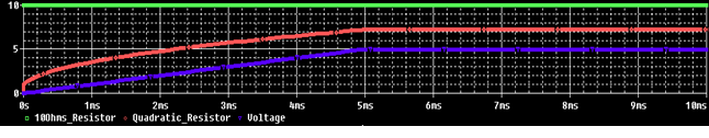
Figure 6: Simulation Results
The PWRS (signed power) function is used instead of I(VSENSE)2 because we want the sign of the voltage across ERES to become negative when the current through VSENSE is negative.
There are a couple of things to watch for when creating nonlinear devices this way. First, all physical impedances have zero current at zero voltage.
Second, one needs to be careful of the asymptotic behavior of the device. It is very easy to create devices which generate power at high voltages. Even though the real circuit may not operate at such voltages, there is nothing to prevent PSpice from finding an unrealistic solution at a high voltage. In general, it is good practice to use the TABLE form to limit the output of devices. For example, here is a constant-power load:
GCONST A B TABLE {100/V(A,B)} = (-100,-100) (100,100)
Where A and B represents the positive and negative terminal nodes of V7.
GCONST tries to dissipate 100 watts of power regardless of the voltage across it. For very small voltages the formula 100÷V(A,B) can lead to unreasonable values of current. The TABLE limits the current to be between -100 and +100 amps.
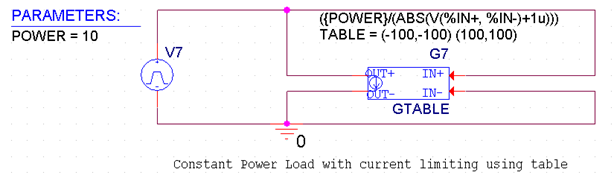
Figure 7: Constant Power Load using table
In power systems, it is common to encounter loads which draw constant power. To model such a load, we can use a voltage dependent current source. A first approximation looks like this:
gload A B value = {pload/v(A,B)}
Where A and B represents the positive and negative terminal nodes of V1.
With this formula, the power = v*i = v(A,B)*(pload/v(A,B)) = pload, as desired.
Unfortunately, this first approximation behaves badly near v = 0. When calculating the bias point for more difficult circuits, PSpice reduces the power supplies. PSpice relies on the assumption that, when the supplies are close enough to 0, all devices in the circuit are turned off. The above formula violates this assumption. Further, it is not a good model of a real constant-power load for low voltages.
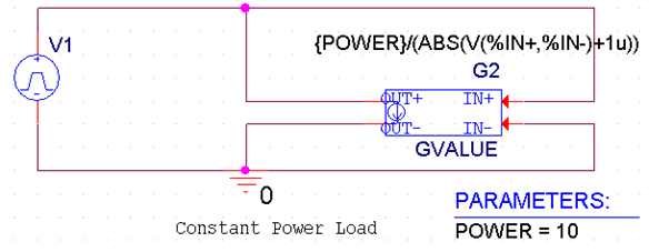
Figure 8: Constant Power Load
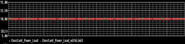
Figure 9: Simulation Results
A real load can only consume constant power over a limited range of applied voltage. When the voltage drops below this range, the load's impedance stops falling. For many loads, a good model is a series connection of two resistances: the fixed minimum resistance and the dynamic constant-power resistance. We can write
Rtotal = Rmin + Rvar = Rmin + v2/P
i = v/Rtotal = v/(Rmin + v2/P) = 1/(Rmin/v + v/P)
For low v, i = v/Rmin. For high v, i = P/v. The corresponding PSpice statement is
gload n1 n2 value = {1/(RMIN/v(n1,n2) + v(n1,n2)/PLOAD}
This device behaves like a resistor of value RMIN at low applied voltages and like a constant-power load at high voltages. The crossover occurs at
Rmin/v = v/P->v2 = RminP->v2/Rmin = P
when the power dissipated in Rmin equals the desired power, P. This is the point of maximum power dissipation into Rmin. For higher voltages the current falls and most of the power is dissipated by Rvar.
This approach can also be used to create frequency-dependent impedances. The main difference is that the LAPLACE or FREQ type is used. For example, a capacitor can be written as:
GCAP A B LAPLACE {V(A,B)} = {s}
The current through GCAP is the integral of V(A,B). However, the LAPLACE device uses much more computer time and memory than does the built-in capacitor (C) device. We recommend the LAPLACE form only for cases where its flexibility is needed. Note that, in general, frequency-dependent impedances have varying phases as well as varying magnitudes of impedance. For example, the formula for a wire with skin effect is:
EWIRE A 4a LAPLACE {I(VSENSE)}={R0 + R1*sqrt(s)}
VSENSE 4a B
The wire's impedance is constant (and real) at low frequencies. At high frequencies, its impedance behaves as the square root of the frequency and becomes half real and half imaginary (that is, it becomes half inductive).
© Copyright 2016 Cadence Design Systems, Inc. All rights reserved. Cadence, the Cadence logo, and Spectre are registered trademarks of Cadence Design Systems, Inc. All others are properties of their respective holders.
Copyright © 2020 Cadence Design Systems, Inc. All rights reserved.